Spatial and temporal parasite dynamics: microhabitat preferences and infection progression of two co-infecting gyrodactylids - Parasites & Vectors

Experimental data

The data used here are from the experimental study of Cable and van Oosterhout [45], subsequently used as the basis of an agent-based model in van Oosterhout [53]. Briefly, cultures of three different Gyrodactylus strains were used to infect three different fish stocks: Ornamental Stock (OS), Lower Aripo River fish (LA) and Upper Aripo River fish (UA); 157 guppies in total, in a full factorial design to give nine different host-parasite combinations, with 13–22 replicates per combination. Two out of the three parasite strains were Gyrodactylus turnbulli, a laboratory-bred strain (Gt3) and a wild turnbulli strain obtained from guppies caught in the Lower Aripo River, Trinidad (Gt), whereas the third strain was G. bullatarudis, also a wild type obtained from hosts in the Lower Aripo River. Both male (68) and female (89) individually isolated guppies were used for the experiment and maintained under constant environmental conditions ($25\pm 0.5 \,^\circ$C; 12h light/12h dark regime). All tanks and containers were kept in a randomised block design to reduce common environmental effects.

The fish considered in the experiment were naive and thus bred under parasite-free conditions. Each fish was then infected with two parasites at time 0, and parasites were counted every 48 h over a 17-day infection period. For each fish, the number of parasites was recorded across eight different body regions (tail fin, lower body, upper body, anal fin, dorsal fin, pelvic fins, pectoral fins and head). Survival data describing the various host infection statuses (remain infected, recovered from the infection or died) over time were extracted from the empirical data for the multi-state modelling. The number of surviving fish (with or without host infection loss) and dead fish across the nine different host-parasite groups over time from days 1 to 17 is tabulated in Appendix 1.

Statistical analyses

Summary

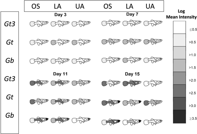
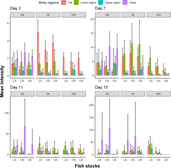
All analyses were carried out using R version 3.6.3 [57]. Images of fish were produced in Gimp software version 2.10.12 [58] and outlined in R. Two graphical summaries of the data were produced. These are available in full in the Additional file 1: Fig. S1 and Additional file 2: Fig. S2, with examples given in Figs. 1 and 2. For the first summary (Fig. 1 and Additional file 1: Fig. S1), the shading represents the log mean intensity of parasites over surviving fish. The number of surviving fish for the nine different host-parasite groups (obtained from the fully crossed design of the three parasite strains and three different host populations) generally decreased (slowly) over time from days 1 to 17 (refer to Appendix 1). For the second graphical summary (Fig. 2 and Additional file 2: Fig. S2), the eight body regions of the fish were recategorized into four: tail, lower region (comprising of the lower body, anal fin, pelvic fins and dorsal fin), upper region (made up of the upper body and pectoral fins) and the head. This re-categorisation allowed us to visually and statistically assess any caudal-rostral preference of the three parasite strains on the three fish stocks more effectively over the study period because of low parasite numbers observed on the fish fins (anal fin, pelvic fins, dorsal fin and pectoral fin).

Multivariate Kruskal-Wallis test for parasite distribution comparison across host body regions

The multivariate Kruskal–Wallis test (MKW) is a multivariate extension of the distribution-free univariate Kruskal-Wallis test [59]. We used it to test the null hypothesis that distribution of parasite number at the four body regions (tail, lower region, upper region and head) is equal for the different host-parasite combinations at each observed time point.

Let $Y_{ij}$ be a vector of the number of parasites at the four body regions for the jth fish from the ith group (host-parasite combination), where $i=1,2,3,\cdots ,9$ and $j=1,2,3,\cdots ,n_{i}$. Let $R_{ij}$ be the rank corresponding to $Y_{ij}$ calculated element-wise (ties are assigned a mean rank) and ${\bar{R}}_{i}=\sum \nolimits _{j=1}^{n_i}{\frac{R_{ij}}{n_i}}$ then $E({\bar{R}}_{i})=m=\frac{n+1}{2}$ under $H_0$; where $n=\sum \nolimits _{i=1}^{9}{n_i}$ is the total number of fish ($n=157$), ${\bar{R}}_{i}$ is the mean rank for each ith group and ${n_i}$ is the number of fish in group i. The vector $U_{i}=(\bar{R}_{i1}-m,\bar{R}_{i2}-m,\bar{R}_{i3}-m,\bar{R}_{i4}-m)^\prime$ denotes the average ranks for the ith group corrected for m for each variate (body regions). The pooled within-group covariance matrix is estimated as

$$\begin{aligned} V=\frac{1}{n-1}\sum _{i=1}^{9}\sum _{j=1}^{n_i}(R_{ij}-m{1})(R_{ij}-m{1})^\prime \end{aligned}$$

(1)

where $R_{ij}=(R_{ij1},R_{ij2},R_{ij3},R_{ij4})^{\prime }$ and $1=(1,1,1,1)^{\prime }$. The MKW test statistic (${\mathcal {W}}$), given as

$$\begin{aligned} {\mathcal {W}}=\sum _{i=1}^{9}{n_i}{U_i}^{\top }{V^{-1}}{U_i} \sim {\chi }^{2}_{k(g-1)}, \end{aligned}$$

(2)

is approximately (asymptotically) chi-squared with $k(g-1)$ degrees of freedom, where $k=4$ and $g=9$ [59]. After performing the MKW, the univariate Kruskal-Wallis test (UKW) was used to further compare the distribution of parasites at each of the four body regions for each parasite strain (Gt3, Gt and Gb) across the fish stocks (OS, LA and UA) at each time point (days 1 to 17). A Bonferroni-Dunn's post-hoc test was finally applied for pairwise comparisons of the parasite distribution between the different parasite-fish combinations over time. The caudal-rostral preference of the three parasite strains on the three fish stocks was statistically inferred from these tests (testing the niche partition hypothesis of Gyrodactylus turnbulli and G. bullatarudis for preferences at the caudal and head regions, respectively).

Multi-state Markov model for gyrodactylid infection progression

Individual fish after being infected can transition among three discrete host states—fish remains infected (state 1), fish alive with loss of infection (state 2) and fish dead (state 3)—over the observation period. Let $\{X_i(t); t \ge 0\}$ be the state of fish i over time. We suppose that $\{X_i(t)\}$ is a time-inhomogeneous Markov chain with transition rate matrix $Q(t)=\{q_{rs}(t)\}$ for $r,s=1,2,3$. For each $i=1,2, \cdots , 157$, we have observations $X_i=(X_{i0},X_{i1},\cdots ,X_{i9})$ at times $t_0=0$, $t_1=1$, $t_2=3$, $\cdots$ and $t_9=17$. The likelihood for the model parameters $\theta =\{q_{rs}(t)\}$ is given as

$$\begin{aligned} L(\theta )=\prod _{i=1}^{157}L_i(\theta |x_i) \end{aligned}$$

(3)

where $L_i(\theta |x_i)$ is the likelihood contribution for each fish i obtained as product of state transition probabilities

$$\begin{aligned} L_i(\theta |x_i)=\prod _{j=1}^{9}p_{x_{ij-1},x_{ij}}(t_{j-1},t_{j}) \end{aligned}$$

(4)

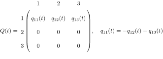
with $p_{x_{ij-1},x_{ij}}(t_{j-1},t_{j})=P\{X_i(t_{j})=x_{ij}|X_i(t_{j-1})=x_{ij-1} \}.$ We assumed that once a fish had lost its infection (state 2) or died (state 3), it could not be reinfected because of the experimental design (move back to state 1) and thus the corresponding rates are 0. Hence, the transition rate matrix Q(t) for the multi-state model with the three discrete host states is given as

where $q_{12}(t)>0$ and $q_{13}(t)>0$ are the rates at which an infected fish loses its infection and dies at time t respectively. Here, we modelled the rate matrix Q(t) as a piecewise constant function with change points $t_1,t_2,\cdots ,t_{8}$. For $t{\in }[t_{j-1},t_j)$, we write $Q(t)=Q_j$. The transition probability matrix is

$$\begin{aligned} P(s,t)= \big (P_{ij}(s,t) \big )_{ij}=(P \big (X(t)=j|X(s)=i \big ) \big )_{ij}=e^{\int _s^{t} Q(u)du} \end{aligned}$$

(5)

The likelihood function for the model parameters is estimated using a maximum likelihood method, fitted using the msm package in R [60].

Estimating the probability of transition and virulence given covariates

We examine how variables such as fish sex, fish size, fish stock and parasite strain may affect the transition rates Q(t). Let $z_i=\{z_{i1},z_{i2},z_{i3}, z_{i4}\}$ be the realized values of the covariates (fish sex, fish size, fish stock and parasite strain) for fish i. Then, the transition rate matrix entries $q_{rs}(t)$ for $r, s= 1, 2, 3$ and $t{\in }[t_{j-1},t_j)$ were taken as

$$\begin{aligned} q_{rs}(t, z_i)={q_{rsj}^{(0)}}{exp(\beta _{rs1}z_{i1} + \beta _{rs2}z_{i2}+ \beta _{rs3}z_{i3}+ \beta _{rs4}z_{i4})} ={q_{rsj}^{(0)}}{exp(\beta _{rs}^{T}{z_i})} \end{aligned}$$

(6)

where ${q_{rsj}^{(0)}}$ is baseline intensity; $\beta _{rs}$ is a parameter vector. The likelihood is then maximized over ${q_{rsj}^{(0)}}$ and the regression coefficients $\beta _{rs}$, for $r=1$ and $s=2,3$. The hazard ratios (HR) corresponding to each covariate are $exp(\beta _{rs})$, for $r=1$ and $s=2,3$. The transition probabilities were estimated from $q_{rs}(t, z_i)$ using Eq. 5. Given the four predictors (fish sex, fish size, fish stock and parasite strain) and two possible transitions from state 1 to either state 2 ($q_{12}$) or state 3 ($q_{13}$) in the proposed multi-state Markov model (defined by Eq. 6), there are $16^2$ (or 256) possible variable permutations or models (which includes transitions independent of the underlying covariates).

A systematic variable and model selection was carried out using both Akaike information criterion (AIC) and Bayesian information criterion (BIC) statistics (due to the relative advantages of the two model selection criteria), where all possible variable permutations or models were considered. The AIC statistic assesses the model's goodness of fit while reducing the complexity of the underlying parameters, whereas the BIC statistics penalise adding more parameters or strongly penalise free parameters compared to the AIC statistic. According to Kuha [61], effective model selection can be achieved by using both AIC and BIC statistics, predominantly to identify models favoured by both criteria, although the study's methodological design, the main research questions and the belief of a true model and its applicability to the study are crucial factors in determining whether to utilise the AIC or BIC [62]. The best model (among identified parsimonious or highly predictive models) was finally chosen based on a likelihood ratio test (LRT) at a 5% significance level. Detailed results on the variable selection for the multi-state model and its R codes (for reproducibility of results) can be found via the GitHub URL link: github.com/twumasiclement/Spatial-Temporal-Parasite-Dynamics.

Let $T_1$ be the time spent in state 1, given that the fish or the process is in state 1 at time 0. Then, the mean sojourn time in state 1 is given as

$$\begin{aligned} E(T_1)= \sum _{j=1}^{\infty } E(T_1|\text {leave in period }j) \times \text {P(leave in period )j}, \end{aligned}$$

(7)

where

$$\begin{aligned} E(T_1\mid \text {leave in period }j)=t_{j-1}+E(S_j|S_j\le t_j-t_{j-1}) \end{aligned}$$

(8)

with

$$\begin{aligned} S_j \sim \exp (q_{12}(j,z_i)+q_{13}(j,z_i)), \end{aligned}$$

and $E(S_j|S_j\le t_j-t_{j-1})$ is given by Eq. 11 according to Theorem 1. In Eq. 7, the probability that the process leaves in period j, denoted by $\text {P(leave in period j)}$, is computed such that

$$\begin{aligned} \text {P(leave in period j)}= \left\{ \begin{array}{ll} P(S_j \le t_j-t_{j-1}),&{} j=1\\ \left[ 1- \sum _{j^{\prime }=1}^{j-1} \text {P(leave in period} j^{\prime }) \right] \times P(S_j \le t_j-t_{j-1}), &{} 2 \le j \le 7\\ 1- \left[ \sum _{j^{\prime }=1}^{7} \text {P(leave in period} j^{\prime }) \right] , &{} j \ge 8 \\ \end{array}\right. \end{aligned}$$

with

$$\begin{aligned} P(S_j\le {t_j-t_{j-1}} )=1-\mathrm{e}^{-({{q_{12}(j,z_i)+q_{13}(j,z_i)})(t_j-t_{j-1})} } \quad \quad \text {for} \quad j \ge 1 \end{aligned}$$

in accordance to Eq. 10 under Theorem 1.

Theorem 1

Let $S_j$ be the time spent by infected fish during period j. Suppose that $S_j \sim \exp \left( q_{12}(j,z_i)+q_{13}(j,z_i) \right)$ with probability density

$$\begin{aligned} f(S_j)= \left[ q_{12}(j,z_i)+q_{13}(j,z_i)\right] \mathrm{e}^{-(q_{12}(j,z_i)+q_{13}(j,z_i))S_j}, \quad S_j>0 \end{aligned}$$

where $q_{12}(j,z_i)$ and $q_{13}(j,z_i)$ are the transition rates from state 1 to state 2 and 3, respectively, given the covariates $z_i$ for fish i, such that

$$\begin{aligned} E(S_j)=\frac{1}{{q_{12}(j,z_i)+q_{13}(j,z_i)}}. \end{aligned}$$

Then,

$$\begin{aligned} E \left[ S_j \mathbbm {1}_{\{S_j \le {t_j-t_{j-1}}\}} \right] =E(S_j) - \left[ t_j-t_{j-1}+E(S_j) \right] \mathrm{e}^{-({{q_{12}(j,z_i)+q_{13}(j,z_i)})(t_j-t_{j-1})} } \end{aligned}$$

(9)

and

$$\begin{aligned} P(S_j\le {t_j-t_{j-1}} )=1-\mathrm{e}^{-({{q_{12}(j,z_i)+q_{13}(j,z_i)})(t_j-t_{j-1})} }. \end{aligned}$$

(10)

For the mathematical proof to Theorem 1, see Appendix 2. From Theorem 1, it can be deduced that

$$\begin{aligned} \begin{aligned} E(S_j|S_j\le t_j-t_{j-1})&=\frac{E \left[ S_j \mathbbm {1}_{\{S_j \le {t_j-t_{j-1}}\}} \right] }{P(S_j\le {t_j-t_{j-1}} )} \\&= \frac{E(S_j) - \left[ t_j-t_{j-1}+E(S_j) \right] \mathrm{e}^{-({{q_{12}(j,z_i)+q_{13}(j,z_i)})(t_j-t_{j-1})} } }{1-\mathrm{e}^{-({{q_{12}(j,z_i)+q_{13}(j,z_i)})(t_j-t_{j-1})} }}, \end{aligned} \end{aligned}$$

(11)

where

$$\begin{aligned} E(S_j)=\frac{1}{{q_{12}(j,z_i)+q_{13}(j,z_i)}}. \end{aligned}$$

Also, given the fish or process is in state 1, then the probability of moving to state 2 or 3 next is given as

$$\begin{aligned}&P(\text {transition from state 1 to s}| \text {leave state 1}) \nonumber \\&\quad =\sum _{j=1}^{\infty }P(\text {transition from state 1 to s}| \text {leave in period }j) \times P(\text {leave in period} j), \end{aligned}$$

(12)

where

$$\begin{aligned} P(\text {transition from state 1 to s}| \text {leave in period }j)=\frac{q_{1s}(j,z_i)}{q_{12}(j,z_i)+q_{13}(j,z_i)} \end{aligned}$$

for $s=2,3$. We assume that $q_{12}(t,z_i)=q_{12}(15,z_i)$ and $q_{13}(t,z_i)=q_{13}(15,z_i)$ for $t \ge 15$.

Threadworm Medicine